Cracking the Code: Ap Statistics Chapter 6 Homework Answers Unveiled
Welcome to our guide on AP Statistics Chapter 6 homework answers! In this article, we will be providing step-by-step solutions to the various exercises you may encounter in your AP Statistics homework assignments for Chapter 6. Chapter 6 focuses on the topic of probability, including concepts such as random variables, probability distributions, and expected values.
Probability is a fundamental concept in statistics that allows us to make predictions and analyze data. It is important to have a solid understanding of probability in order to effectively interpret and analyze statistical data. In this chapter, you will learn about probability distributions, which describe the likelihood of different outcomes in a random experiment. You will also explore the concept of expected value, which allows us to calculate the average outcome of a random experiment.
Throughout this chapter, you will work on a variety of exercises to reinforce your understanding of these concepts. These exercises may involve solving probability problems, calculating expected values, and interpreting probability distributions. Our goal is to provide detailed solutions to these exercises, helping you to gain a deeper understanding of the material and excel in your AP Statistics coursework.
So whether you’re a student looking for help with your AP Statistics homework or a teacher seeking additional resources for your lesson plans, this article is here to assist you. We hope that our step-by-step solutions will clarify any confusion and enable you to confidently tackle the exercises in Chapter 6 of your AP Statistics textbook.
Understanding AP Statistics Chapter 6 Homework Answers
The AP Statistics Chapter 6 focuses on the topic of probability. In this chapter, students learn about the concept of probability, different types of probability, and how to calculate probabilities using various techniques. The chapter also covers the important topic of random variables and their probability distributions.
Completing the homework for Chapter 6 helps students reinforce their understanding of probability concepts and practice applying them to real-world scenarios. The homework answers provide a valuable tool for students to check their work and evaluate their understanding of the material. By reviewing the answers, students can identify any mistakes, misconceptions, or areas of confusion they may have had while completing the assignments.
The homework answers for Chapter 6 typically include step-by-step explanations and solutions to the problems. They may also include additional examples or practice questions to further reinforce the concepts covered in the chapter. By studying and understanding the homework answers, students can gain a deeper understanding of the material and improve their overall performance in the class.
It is important for students to actively engage with the homework answers and not just rely on them as a way to complete their assignments. By carefully reviewing the solutions and explanations, students can develop critical thinking skills and problem-solving strategies that will benefit them not only in this chapter but also in future chapters and in real-life applications of probability.
Overall, understanding the AP Statistics Chapter 6 homework answers is crucial for students to master the concepts of probability and enhance their performance in the course. By using the answers as a learning tool, students can identify areas of weakness, clarify any confusion, and improve their ability to solve problems related to probability.
Exploring the Types of Data
Data is the foundation of statistics, and understanding the different types of data is crucial for any statistical analysis. When conducting research or analyzing a problem, it is important to identify the type of data you are working with. In statistics, data can be categorized into two main types: quantitative and qualitative.
Quantitative Data:
Quantitative data is numerical data that represents quantities or measurements. This type of data can be further divided into two subtypes: discrete and continuous.
- Discrete data: Discrete data consists of whole numbers or values that are countable and finite. Examples of discrete data include the number of siblings a person has, the number of cars in a parking lot, or the number of students in a class.
- Continuous data: Continuous data, on the other hand, can take on any value within a specific range. It is measured on a continuous scale and usually involves some form of measurement. Examples of continuous data include the height of individuals, the weight of objects, or the temperature of a room.
Qualitative Data:
Qualitative data, also referred to as categorical data, is descriptive in nature and represents qualities or characteristics. It can be classified into different categories or groups. This type of data does not have numeric values and cannot be measured. Qualitative data can be further divided into two subtypes: nominal and ordinal.
- Nominal data: Nominal data consists of categories or labels with no specific order. Examples of nominal data include gender (male or female), eye color (blue, brown, green), or marital status (single, married, divorced).
- Ordinal data: Ordinal data also consists of categories, but they have a specific order or ranking. Examples of ordinal data include ratings for a movie (excellent, good, fair, poor), education levels (high school, college, graduate), or satisfaction levels (very satisfied, satisfied, dissatisfied).
Understanding the different types of data is essential for selecting the appropriate statistical analysis methods, as different types of data require different statistical techniques. By identifying and categorizing the data correctly, researchers can gain valuable insights and draw meaningful conclusions from their analyses.
Understanding the Measures of Center and Variation
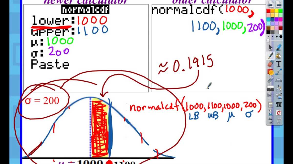
Measures of center and variation are essential statistical tools that help us understand the distribution and variability of data. In statistics, measures of center refer to the values that represent the “center” or “typical” value of a dataset. These measures provide insights into the central tendency of the data and can help us compare different datasets.
One commonly used measure of center is the mean, which is calculated by summing all the values in a dataset and dividing the sum by the total number of values. The mean provides an average value that represents the center of the data. Another measure of center is the median, which is the middle value when the dataset is ordered from smallest to largest. The median is less affected by extreme values and can be a better representation of the “typical” value when the dataset is skewed.
In addition to measures of center, measures of variation help us understand the spread or variability of the data. One popular measure of variation is the standard deviation, which quantifies the average distance between each data point and the mean. A larger standard deviation indicates greater variation in the data, while a smaller standard deviation suggests less variability. Another measure of variation is the range, which is simply the difference between the largest and smallest values in the dataset.
Understanding and analyzing the measures of center and variation is crucial in various fields of study, including finance, economics, and social sciences. These measures help us summarize and interpret data, identify outliers, and make informed decisions based on the characteristics of the dataset.
Learning about the Normal Distribution
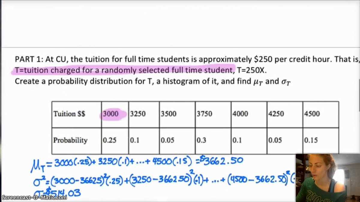
The normal distribution, also known as the Gaussian distribution, is a commonly encountered continuous probability distribution. It is characterized by a bell-shaped curve that is symmetrical, with the mean, median, and mode all being equal. Understanding the properties and characteristics of the normal distribution is essential in statistics, as it is widely used to model various natural and social phenomena.
One important property of the normal distribution is its mean and standard deviation. The mean, denoted as µ, represents the center of the distribution, while the standard deviation, denoted as σ, controls the spread or variability of the distribution. The normal distribution is fully characterized by these two parameters. Additionally, for any given normal distribution, the area under the curve is equal to 1.
Properties of the normal distribution:
- The normal distribution is bell-shaped and symmetrical.
- The mean, median, and mode of the distribution are equal.
- The total area under the curve is equal to 1.
- The distribution is fully characterized by the mean and standard deviation.
The normal distribution is widely used in statistics due to its numerous applications. For example, it is commonly used to approximate the distribution of a large sample mean or sum, as well as to determine confidence intervals and conduct hypothesis testing. It is also frequently used in the field of quality control, as it provides a useful reference distribution for comparing measurements or process outputs.
Understanding the normal distribution and its properties is fundamental in statistics, as it lays the foundation for various statistical techniques and concepts. By studying and analyzing data using the normal distribution, statisticians can gain valuable insights into the underlying population and make informed decisions based on the observations.
Conducting Hypothesis Tests
In statistics, hypothesis tests are used to make inferences about population parameters based on sample data. These tests involve formulating a null hypothesis and an alternative hypothesis, and then collecting and analyzing the data to determine the likelihood of observing the data given the null hypothesis is true.
The first step in conducting a hypothesis test is to clearly state the null and alternative hypotheses. The null hypothesis represents the status quo or the default assumption, while the alternative hypothesis represents what the researcher is trying to prove or find evidence for.
Once the hypotheses are defined, the next step is to collect sample data and calculate a test statistic. The test statistic is a numerical value that summarizes the evidence against the null hypothesis. The choice of test statistic depends on the type of data and the specific hypothesis being tested.
After calculating the test statistic, the next step is to determine the p-value. The p-value is the probability of obtaining a test statistic as extreme as or more extreme than the one calculated, assuming the null hypothesis is true. A small p-value suggests strong evidence against the null hypothesis.
Finally, a decision is made based on the p-value and a predetermined significance level, often denoted as alpha. If the p-value is less than alpha, the null hypothesis is rejected in favor of the alternative hypothesis. If the p-value is greater than alpha, there is not enough evidence to reject the null hypothesis.
In summary, conducting hypothesis tests involves formulating and stating the null and alternative hypotheses, collecting and analyzing sample data to calculate a test statistic and p-value, and making a decision based on the p-value and significance level.
Analyzing Two-Way Tables
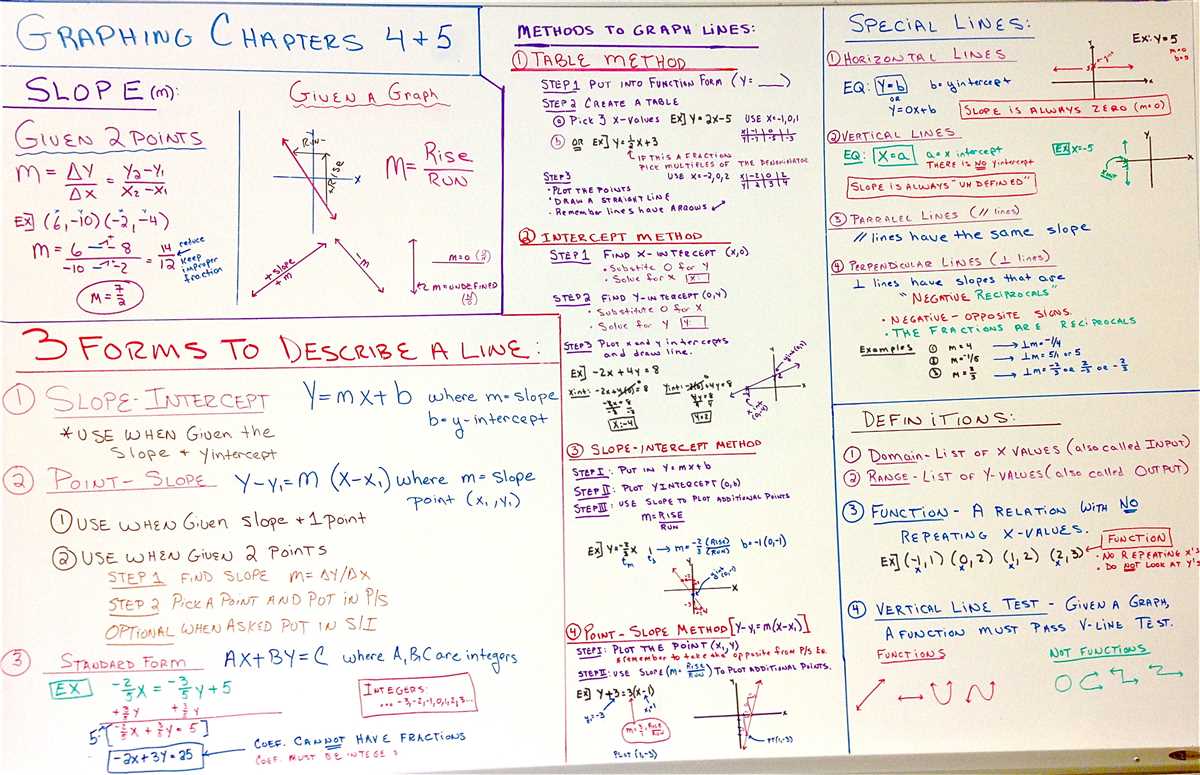
Two-way tables, also known as contingency tables, are used to analyze and summarize categorical data. They provide a way to organize data into rows and columns, allowing for comparison and examination of relationships between two different categorical variables.
In a two-way table, each cell represents a combination of values from the two categorical variables. The rows represent one variable, while the columns represent the other variable. The numbers in the cells represent the frequency or count of observations falling into each combination.
With two-way tables, we can calculate various statistics and measures to further analyze the data. For example, we can calculate row and column percentages to understand the distribution of one variable within each category of the other variable. This can help us identify any patterns or associations between the two variables.
Additionally, we can perform chi-square tests of independence on two-way tables to determine if there is a significant association between the variables. This test helps us determine if the observed frequencies differ significantly from what would be expected if the variables were independent of each other.
Two-way tables are widely used in various fields, such as market research, social sciences, and public health, to analyze and interpret categorical data. They provide a visual representation and allow for deeper exploration of the relationship between variables. By using statistical techniques and measures, we can uncover valuable insights and make informed decisions based on the data.
Conclusion:
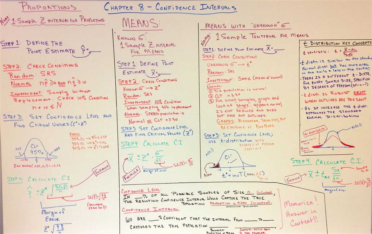
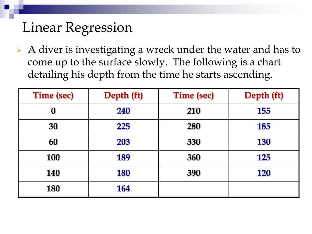
In conclusion, interpreting linear regression and correlation is essential for understanding the relationship between two variables. Linear regression helps us predict the value of one variable based on the other, while correlation measures the strength and direction of the relationship.
Through regression analysis, we can determine the equation of a line that best fits the data points, and use this equation to make predictions. The slope of the regression line represents the change in the response variable for a one unit increase in the predictor variable, while the y-intercept represents the predicted value when the predictor variable is zero.
Correlation, on the other hand, allows us to determine the direction and strength of the relationship between two variables. A correlation coefficient close to +1 indicates a strong positive relationship, while a coefficient close to -1 indicates a strong negative relationship. A coefficient close to zero suggests little to no relationship.
It is important to note that correlation does not imply causation. Just because two variables are correlated does not mean that one variable causes the other to change. Other factors may be at play, and further analysis is needed to establish causality.
Overall, interpreting linear regression and correlation allows us to gain insights into the relationship between variables and make predictions based on the data. It is a fundamental tool in statistics and can be widely applied in various fields such as economics, social sciences, and marketing.