Mastering Chapter 7: Your Ultimate Guide to Acing the Algebra 1 Test
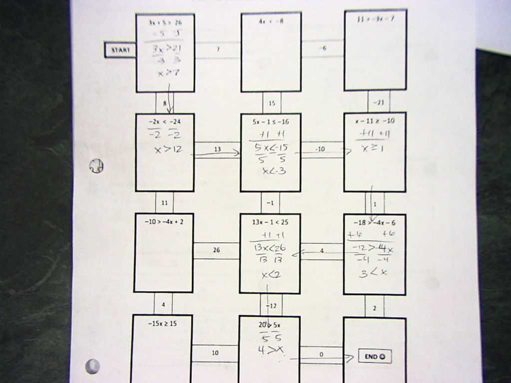
Algebra 1 is a fundamental subject in mathematics that lays the foundation for more advanced mathematical concepts. Chapter 7 specifically focuses on various topics, including solving systems of linear equations and inequalities, graphing linear equations, and quadratic functions. To assess students’ understanding and mastery of these concepts, a Chapter 7 Algebra 1 test is often administered.
This comprehensive test evaluates students’ ability to apply algebraic principles and concepts to solve real-world problems. It tests their knowledge of solving equations and inequalities, interpreting and analyzing graphs, and understanding the properties of quadratic functions. The test may consist of multiple-choice questions, word problems, and free-response questions that require students to demonstrate their understanding and problem-solving skills.
The Chapter 7 Algebra 1 test serves not only as an assessment tool but also as a means for students to gauge their own understanding of the material. It allows them to identify areas of strength and areas that require further review and practice. Additionally, the test provides teachers with valuable insights into students’ comprehension levels, enabling them to modify teaching approaches and provide targeted support to ensure student success.
Chapter 7 Algebra 1 Test: Key Topics to Know
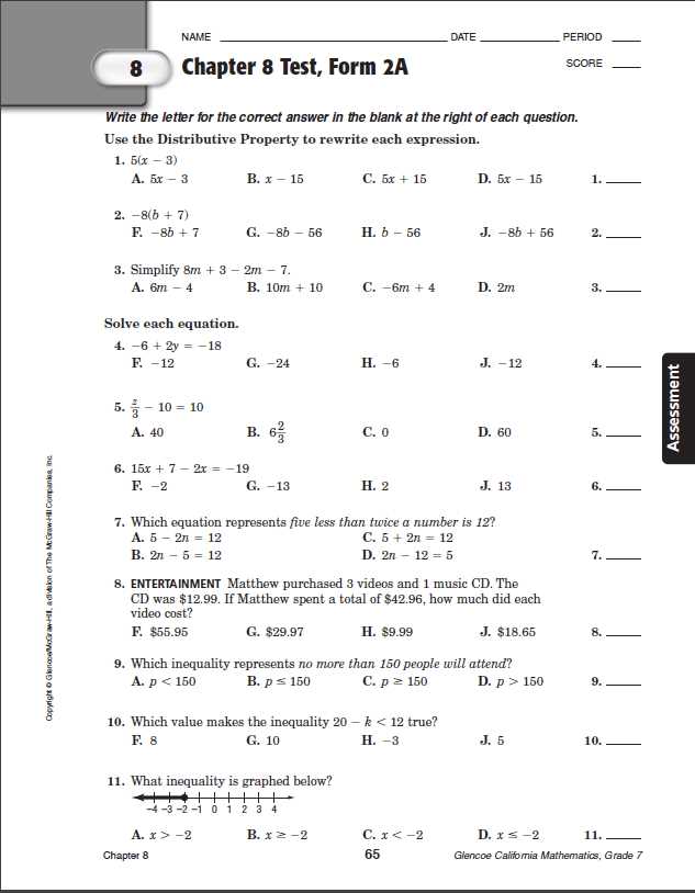
Preparing for a chapter 7 algebra 1 test requires a solid understanding of several key topics. These topics are essential for success on the test and in future algebra courses. It is important to review these topics thoroughly and practice solving problems related to each concept.
1. Linear Equations: Linear equations play a crucial role in algebra. Understanding how to write a linear equation given a slope and a point or two points, how to graph linear equations, and how to solve systems of linear equations is essential for success on the chapter 7 algebra 1 test.
2. Quadratic Equations: Quadratic equations involve variables raised to the power of 2. It is important to understand how to solve quadratic equations by factoring, using the quadratic formula, or completing the square. Additionally, understanding how to graph quadratic equations and finding the vertex, axis of symmetry, and x-intercepts is crucial for answering test questions related to this topic.
3. Functions: Functions involve a relationship between two sets of numbers. Understanding the concept of a function, how to evaluate functions, how to find the domain and range of a function, and how to graph functions is important for success on the chapter 7 algebra 1 test.
4. Exponents and Radicals: Exponents and radicals involve manipulating numbers raised to a power or rooted. It is important to understand the rules of exponents, how to simplify expressions with exponents, and how to solve equations involving exponents and radicals.
5. Polynomial Operations: Polynomial operations involve adding, subtracting, multiplying, and dividing polynomials. Understanding how to perform these operations, simplify polynomial expressions, and solve equations involving polynomials is crucial for success on the test.
6. Inequalities: Inequalities involve comparing two expressions using the symbols <, >, ≤, or ≥. It is important to understand how to solve and graph inequalities, as well as how to solve systems of inequalities.
7. Word Problems: The chapter 7 algebra 1 test is likely to include word problems that require translating real-life situations into algebraic expressions and equations. It is important to practice solving word problems and understanding how to interpret the information given in the problem.
By thoroughly understanding and practicing these key topics, students can confidently approach the chapter 7 algebra 1 test and achieve success.
Solving Linear Equations
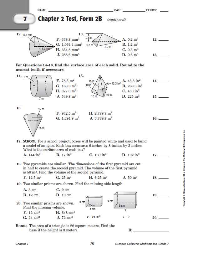
Linear equations are a fundamental concept in algebra that involve finding the value of an unknown variable. They are called “linear” because the highest power of the variable in the equation is 1. Solving linear equations requires applying specific algebraic steps to isolate the variable and find its value.
One of the first steps in solving a linear equation is to combine like terms on both sides of the equation. This involves adding or subtracting terms with the same variable and exponent. By simplifying the equation in this way, it becomes easier to isolate the variable on one side of the equation.
Once like terms have been combined, the next step is to isolate the variable by performing inverse operations. This usually involves adding or subtracting constants or variables from both sides of the equation. The goal is to eventually have the variable by itself on one side of the equation.
In some cases, it may be necessary to use the distributive property or combine like terms again after isolating the variable. The final step is to divide both sides of the equation by the coefficient of the variable to find its value. It’s important to remember that whatever operation is performed on one side of the equation must also be performed on the other side to maintain the equality of the equation.
Solving linear equations is a fundamental skill in algebra and provides a foundation for solving more complex equations and systems of equations. By understanding the steps and concepts involved in solving linear equations, students can develop their problem-solving and critical-thinking skills.
Graphing Linear Equations
Graphing linear equations is an essential skill in algebra. It allows us to visually represent the relationship between two variables. The graph of a linear equation is a straight line, and by plotting points on this line, we can easily determine its slope and y-intercept. This information is crucial in understanding the behavior of the equation and analyzing its solutions.
When graphing a linear equation, we use the slope-intercept form, which is y = mx + b. In this equation, m represents the slope of the line, and b represents the y-intercept, the point where the line crosses the y-axis. To graph the equation, we can start by plotting the y-intercept (0, b), and then use the slope to find other points. The slope tells us how steep or flat the line is. For every increase of 1 unit in the x-direction, the line will increase or decrease by the value of the slope.
To further analyze the graph of a linear equation, we can determine its x-intercept by setting y = 0 and solving for x. The x-intercept is the point where the line crosses the x-axis. Additionally, we can calculate the slope using the y-values of any two points on the line. The slope is found by taking the difference in y-values and dividing it by the difference in x-values. Understanding these aspects of graphing linear equations helps us interpret the equation’s meaning and solve real-world problems.
Summary:
- Graphing linear equations helps us visualize the relationship between two variables.
- The slope-intercept form y = mx + b is used to graph linear equations.
- The slope represents the steepness of the line, and the y-intercept is the point where it crosses the y-axis.
- The x-intercept is found by setting y = 0 and solving for x.
- The slope can be calculated using the difference in y-values and x-values of any two points on the line.
Systems of Linear Equations
A system of linear equations refers to a set of equations that involve two or more unknown variables. These equations can be written in the form of ax + by + cz + … = d, where a, b, c, and so on, are the coefficients, and x, y, z, and so on, are the variables.
Solving a system of linear equations involves finding the values of the variables that satisfy all the equations simultaneously. This can be achieved through various methods, such as substitution, elimination, or matrix operations. The solution to a system of linear equations can be a unique solution, infinitely many solutions, or no solution at all.
One method for solving systems of linear equations is substitution. This involves solving one equation for one variable and then substituting that expression into the other equations. The goal is to eliminate one variable and reduce the system to a single equation with one variable. This method is useful when one equation is already solved for a variable or when one equation is relatively simple to solve.
Another method for solving systems of linear equations is elimination. This involves adding or subtracting the equations in a way that eliminates one of the variables. The goal is to reduce the system to a single equation with one variable. This method is useful when the coefficients of one variable in the equations are the same or multiples of each other.
Systems of linear equations have many real-life applications, such as solving problems involving unknown quantities, balancing chemical equations, or predicting future trends in data analysis. Being able to solve these systems is an important skill in algebra and can be used in various fields such as engineering, economics, and physics.
Quadratic Functions

A quadratic function is a polynomial function of the second degree. It can be written in the form f(x) = ax^2 + bx + c, where a, b, and c are constants and a ≠ 0. The graph of a quadratic function is a parabola, which can open upwards or downwards depending on the value of a.
Quadratic functions have several important properties. The vertex of the parabola is the point where the function reaches its maximum or minimum value. It is given by the formula x = -b/2a. The axis of symmetry is a vertical line passing through the vertex. The y-intercept is the point where the parabola intersects the y-axis, and it can be found by evaluating the function at x = 0.
The solutions of a quadratic equation, also known as the roots or zeros of the function, can be found by factoring, completing the square, or using the quadratic formula. The quadratic formula states that if ax^2 + bx + c = 0, then the solutions are given by:
| x = | -b + √(b^2 – 4ac) | or | -b – √(b^2 – 4ac) |
|---|---|---|---|
| 2a | 2a |
Quadratic functions are used to model many real-life situations, such as the trajectory of a projectile, the growth of a population, or the cost and revenue functions in economics. They are also important in calculus as they are used to find the maximum and minimum values of functions.
Radical Expressions and Equations
Radical expressions and equations play a key role in algebra 1 and are an important topic covered in the Chapter 7 test. A radical expression is an expression that contains a square root or other nth root. These expressions can be simplified by finding the square root or nth root of a number. The simplified form of a radical expression can help solve equations or simplify complicated mathematical expressions.
When working with radical expressions, it is important to understand the properties of radicals. One property is the product property, which states that the square root of a product is equal to the product of the square roots. Another property is the quotient property, which states that the square root of a quotient is equal to the quotient of the square roots. These properties can be used to simplify and solve equations involving radical expressions.
Radical equations are equations that contain a radical expression. Solving radical equations involves isolating the radical expression and then squaring both sides of the equation to eliminate the radical. However, it is important to note that squaring both sides of an equation may introduce extraneous solutions, which are solutions that do not satisfy the original equation. Therefore, it is necessary to check the solutions obtained from solving radical equations to ensure their validity.
Overall, understanding radical expressions and equations is essential in algebra 1 and is a fundamental concept tested in Chapter 7. By mastering the properties of radicals and the techniques for solving radical equations, students can confidently solve problems involving these types of expressions and equations.
Exponential Functions
An exponential function is a type of mathematical function in which the independent variable appears as an exponent. It can be represented by the equation y = a * b^x, where a and b are constants, and x is the independent variable. Exponential functions can be used to model various real-world phenomena, such as population growth, compound interest, and radioactive decay.
Exponential functions have several key properties:
- As the value of x increases, the value of y increases exponentially.
- Exponential functions have a constant ratio between consecutive outputs, known as the “common ratio”.
- Exponential functions can have a horizontal asymptote, which the graph approaches but never reaches.
- The graph of an exponential function is always a curve that starts at the y-intercept and increases or decreases rapidly.
In this chapter, we have learned how to graph exponential functions, find their domain and range, and solve exponential equations. We have also explored the concepts of growth and decay factors, and how they relate to the common ratio of an exponential function.
Overall, exponential functions are a powerful tool in mathematics and have wide-ranging applications in various fields. Understanding their properties and how to work with them is essential for solving real-world problems and analyzing exponential phenomena.