Master Algebra 1 Chapter 8: Check Your Answers with this Comprehensive Review
Algebra 1 is a fundamental course in high school mathematics that introduces students to the world of variables, equations, and functions. Chapter 8 is a crucial part of the curriculum, focusing on systems of linear equations and inequalities. Mastering this chapter is essential for students to successfully move on to more advanced topics in algebra and beyond.
In this article, we will provide a comprehensive guide to the answers for the Chapter 8 review in Algebra 1. Our goal is to help students gain a deeper understanding of the concepts covered in this chapter and ensure they can confidently solve problems involving systems of equations and inequalities.
We will start by discussing key concepts such as the different methods for solving systems of equations, including graphing, substitution, and elimination. We will also explore how to identify the number of solutions a system has and how to interpret the solution in the context of the problem. Additionally, we will cover solving systems of inequalities and the connection between graphical representations and algebraic solutions.
Throughout the article, we will provide step-by-step explanations for each problem in the Chapter 8 review, ensuring students have a clear understanding of the solution process. By the end of this guide, students will have a solid foundation in solving systems of linear equations and inequalities, enabling them to excel in their algebra studies and other math-related disciplines.
Algebra 1 Chapter 8 Review Answers
In this review of Algebra 1 Chapter 8, we will go through some of the key concepts and problems that were covered in the chapter. We will provide the answers to the review questions, which will help you assess your understanding of the material.
1. Simplify the following expressions:
- a) 3x + 2y – x + 4y = 2x + 6y
- b) 5(x + 3) – (2x – 4) = 3x + 17
- c) 2(x – 4) + 3(2x + 5) = 11x + 2
2. Solve the following equations:
- a) 5x + 6 = 21 => x = 3
- b) 2(4x – 1) = 18 => x = 5
- c) 3x + 7 = 4x – 2 => x = 9
3. Find the slope and y-intercept of the following lines:
- a) 2x + 3y = 9 => slope = -2/3, y-intercept = 3
- b) 4x – 5y = 12 => slope = 4/5, y-intercept = -12/5
- c) 3y = 2x + 6 => slope = 2/3, y-intercept = 2
4. Graph the following inequalities:
- a) y < 2x + 3 - This is a dotted line with a shaded area below the line.
- b) y ≥ -x + 2 – This is a solid line with a shaded area above the line.
- c) 2x – 3y > 6 – This is a dotted line with a shaded area above the line.
These are just a few examples of the types of problems covered in Algebra 1 Chapter 8. By reviewing the answers to these questions, you can better understand the concepts and gain confidence in your algebra skills.
Solving Linear Equations
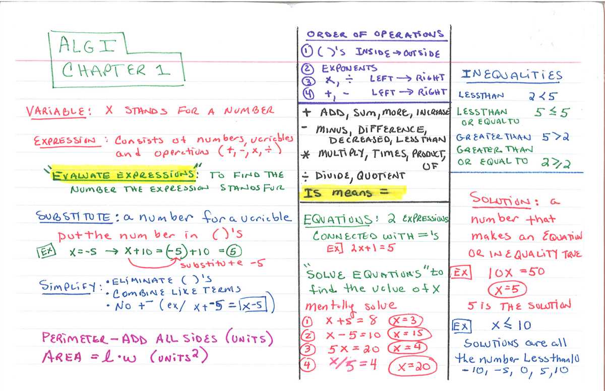
Linear equations are equations that can be written in the form Ax + B = 0, where A and B are constants and x is the variable. Solving linear equations involves finding the value of the variable that makes the equation true. This is done by performing various operations on the equation to isolate the variable on one side.
One common method for solving linear equations is by using the properties of equality. This involves performing the same operation to both sides of the equation in order to maintain equality. For example, if we have the equation 2x + 3 = 9, we can subtract 3 from both sides to get 2x = 6. Then, by dividing both sides by 2, we find that x = 3.
Another method for solving linear equations is by using the inverse operations. Multiplication and division are inverse operations, as well as addition and subtraction. By applying the inverse operation to eliminate a term from one side of the equation, we can then solve for the variable. For example, if we have the equation 5x – 6 = 9, we can add 6 to both sides to get 5x = 15. Then, by dividing both sides by 5, we find that x = 3.
In summary, solving linear equations involves manipulating the equation using the properties of equality or inverse operations to isolate the variable and find its value. This allows us to find the solution to the equation and determine the value of the variable that makes the equation true.
Graphing Linear Equations
In Algebra 1, one of the fundamental skills students learn is how to graph linear equations. Graphing linear equations allows us to visualize relationships between variables and identify important characteristics of a linear equation, such as its slope and y-intercept.
A linear equation is an equation that represents a straight line on a graph. It can be expressed in the form y = mx + b, where m is the slope of the line and b is the y-intercept. The slope of a line determines its steepness, while the y-intercept is the point where the line crosses the y-axis.
To graph a linear equation, we typically start by identifying the y-intercept and plotting that point on the graph. Then, using the slope, we can find additional points to plot, typically by using the rise over run method. This involves moving up or down by the slope’s numerator (rise) and right or left by the slope’s denominator (run) from the y-intercept.
Once we have a few points plotted, we can draw a straight line through them to represent the linear equation. This line will extend infinitely in both directions, representing all possible solutions to the equation.
Graphing linear equations is an important skill in algebra and serves as a foundation for other topics, such as solving systems of equations and understanding inequalities. It allows us to visually analyze the relationship between variables and make predictions based on the graph.
Overall, graphing linear equations is a valuable tool for understanding and visualizing the relationships between variables. It helps us analyze patterns, interpret data, and solve real-world problems. By mastering this skill, students can develop a strong foundation in algebra and pave the way for success in higher-level math courses.
Systems of Linear Equations
A system of linear equations consists of two or more equations with the same set of variables. The goal is to find the values of the variables that satisfy all the equations in the system. This involves finding the solution set, which is the set of all possible values for the variables that satisfy the equations.
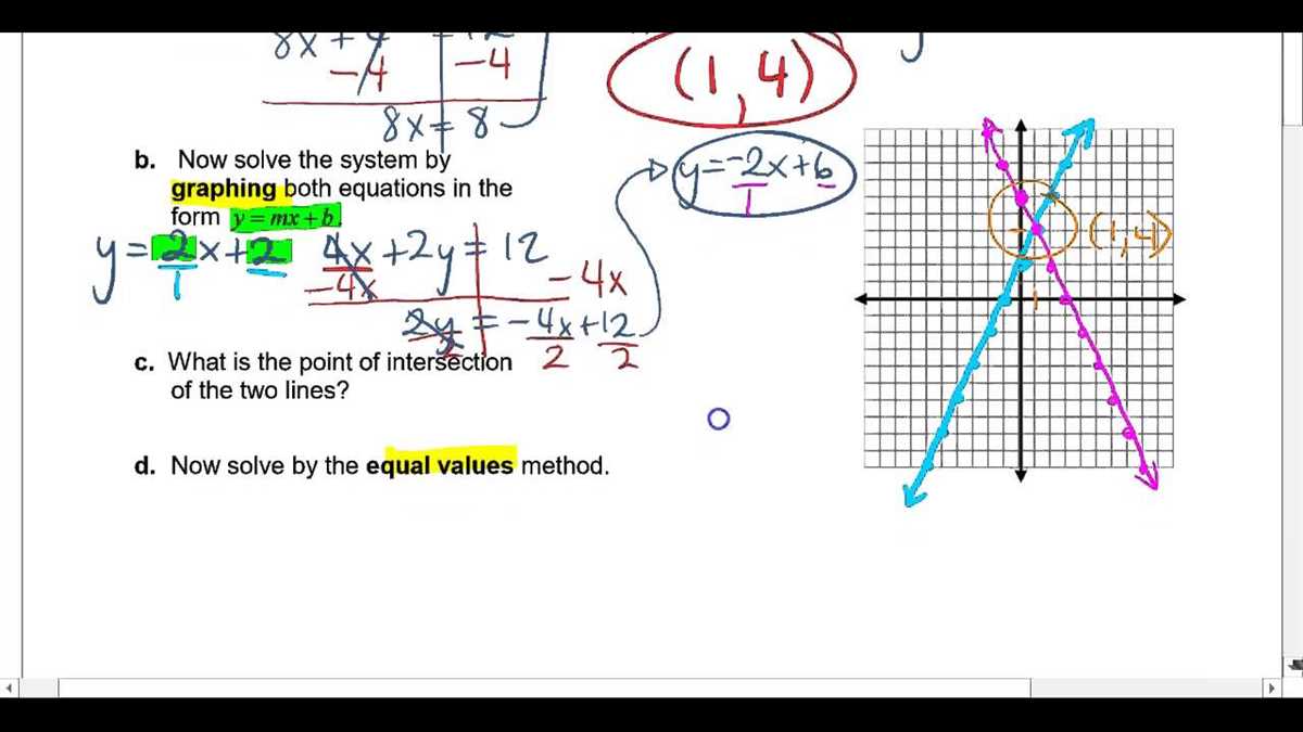
There are several methods for solving systems of linear equations, including graphing, substitution, and elimination. Graphing involves graphing each equation on the same coordinate plane and finding the point or points of intersection. Substitution involves solving one equation for one variable and substituting that expression into the other equation. Elimination involves manipulating the equations to eliminate one variable, usually by adding or subtracting the equations.
Example:
Consider the system of equations:
- 2x + 3y = 8
- 4x – 3y = 10
We can solve this system of equations by adding the two equations:
| 2x + 3y | = 8 |
| + (4x – 3y) | = 10 |
| 6x | = 18 |
| x | = 3 |
Substituting the value of x into one of the original equations, we find:
| 2(3) + 3y | = 8 |
| 6 + 3y | = 8 |
| 3y | = 2 |
| y | = 2/3 |
The solution to the system of equations is x = 3 and y = 2/3.
In conclusion, systems of linear equations involve finding the values of variables that satisfy multiple equations. Various methods can be used to solve these systems, such as graphing, substitution, and elimination. The solution set is the set of all possible values for the variables that satisfy the equations.
Exponents and Exponential Functions

In algebra, exponents are used to represent repeated multiplication of a base number. An exponent is a small number written above and to the right of a base number, indicating how many times the base should be multiplied by itself.
Exponential functions are functions in the form of f(x) = a^x, where “a” is the base and “x” is the exponent. These functions have distinct characteristics, such as exponential growth or decay, which can be represented graphically.
Exponent Rules:
- An exponent of 0 results in 1: a^0 = 1
- An exponent of 1 does not change the value of the base: a^1 = a
- When multiplying two numbers with the same base, add their exponents: a^m * a^n = a^(m + n)
- When dividing two numbers with the same base, subtract their exponents: a^m / a^n = a^(m – n)
Exponential Growth and Decay:
Exponential functions with a base greater than 1 represent exponential growth, while those with a base between 0 and 1 represent exponential decay. These functions can be graphed to visually represent their growth or decay patterns.
| x | f(x) = 2^x | f(x) = (1/2)^x |
|---|---|---|
| 0 | 1 | 1 |
| 1 | 2 | 1/2 |
| 2 | 4 | 1/4 |
| 3 | 8 | 1/8 |
The table above shows the values of x and the corresponding y-values for exponential functions with a base of 2 and 1/2. As x increases, the values of the exponential function with a base of 2 exponentially grow, while the values of the exponential function with a base of 1/2 exponentially decay.
Understanding exponents and exponential functions is essential in mathematics and has numerous applications in fields such as finance, science, and engineering.
Polynomials and Factoring
Polynomials are algebraic expressions that consist of variables and coefficients, combined using addition, subtraction, multiplication, and exponentiation. They can have different degrees, which is determined by the highest power of the variable in the expression. Polynomials are widely used in various mathematical applications, including algebra, calculus, and statistics.
Factoring is the process of finding the factors of a polynomial, breaking it down into simpler terms. This is important in simplifying expressions, solving equations, and determining the zeros or roots of a polynomial. Factoring is also useful in graphing polynomials, as it reveals important information about the function’s behavior, such as its x-intercepts and multiplicity.
When factoring a polynomial, the goal is to break it down into its irreducible components. This often involves identifying common factors, using methods like the greatest common factor (GCF) or factoring by grouping. Other techniques for factoring include the difference of squares, perfect square trinomials, and the sum/difference of cubes formulas.
Examples:
- Factoring the polynomial 2x^2 + 5x + 2 can be done by finding two numbers that multiply to give 2 and add up to 5. In this case, the factors are 1 and 2, so the polynomial can be factored as (2x + 1)(x + 2).
- The polynomial x^3 – 8 can be factored as the difference of cubes by using the formula a^3 – b^3 = (a – b)(a^2 + ab + b^2). In this case, it becomes (x – 2)(x^2 + 2x + 4).
Factoring polynomials is an important skill in algebra, as it allows for the simplification and solution of various mathematical problems. It also provides insights into the behavior and properties of polynomial functions. Understanding and proficiency in factoring can greatly enhance one’s ability to work with algebraic expressions and equations.
Quadratic Equations

In conclusion, understanding and solving quadratic equations is an essential skill in algebra. Quadratic equations have many real-world applications and are used in various fields, including physics, engineering, and economics. By learning about quadratic equations, we can analyze and solve problems that involve finding the maximum or minimum value, determining the shape of a parabola, and finding the roots or solutions.
Throughout this chapter review, we have covered the key concepts related to quadratic equations, including factoring, completing the square, and using the quadratic formula. We have also practiced solving quadratic equations using these techniques and determining the characteristics of the graphs of quadratic functions. It is important to remember that practice and familiarity with these concepts are crucial to mastering the topic of quadratic equations.
By mastering quadratic equations, we are equipped with a powerful tool that allows us to model and solve complex real-world problems. Whether it’s predicting the trajectory of a projectile, analyzing the profit and cost functions in business, or optimizing a design, quadratic equations provide us with the necessary mathematical framework to tackle these challenges. With further practice and application, we can continue to improve our understanding and proficiency in solving quadratic equations.